Predictable Scale: Part I — Optimal Hyperparameter Scaling Law in Large Language Model Pretraining

Houyi Li^1,2 Wenzhen Zheng¹ Jingcheng Hu^1,3 Qiufeng Wang¹ Hanshan Zhang¹ Zili Wang¹

Shijie Xuyang^1,2 Yuantao Fan¹ Shuigeng Zhou² Xiangyu Zhang^1,4 Daxin Jiang¹

¹StepFun ²Fudan University ³Tsinghua University ⁴Megvii Technology

**Figure 1. The hyperparameter space for models with 400M parameters trained on 40B tokens (left) and 1B parameters trained on 100B tokens (right).** All contour lines shown here represent the genuinely converged Train Smooth Loss obtained from small models trained from scratch. The contour lines in the two figures respectively originate from two groups totaling 240 small models with different hyperparameters (Grid Search) trained end-to-end. The Global Minimum is derived from the 120 small models as the one with the minimal final Train Smooth Loss. The contour lines illustrate the relative distance from the Global Minimum in terms of the final loss. Data points exceeding +2% are excluded from the visualization. All mentioned methods have been converted to predict OptimalToken-Wise BatchSize.

Abstract

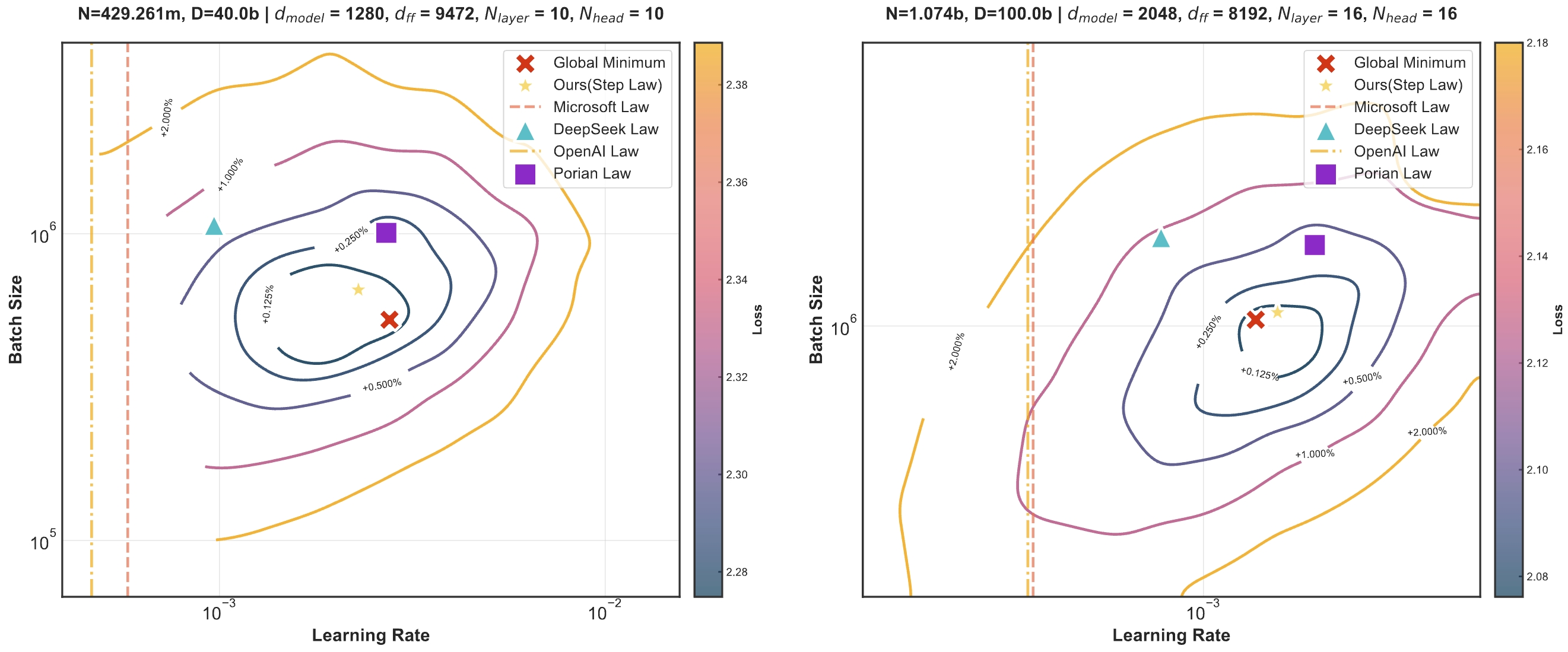
We first present the unified optimal hyperparameter scaling laws, termed Step Law, that generalizes across diverse model shapes, architectures, and data distributions.

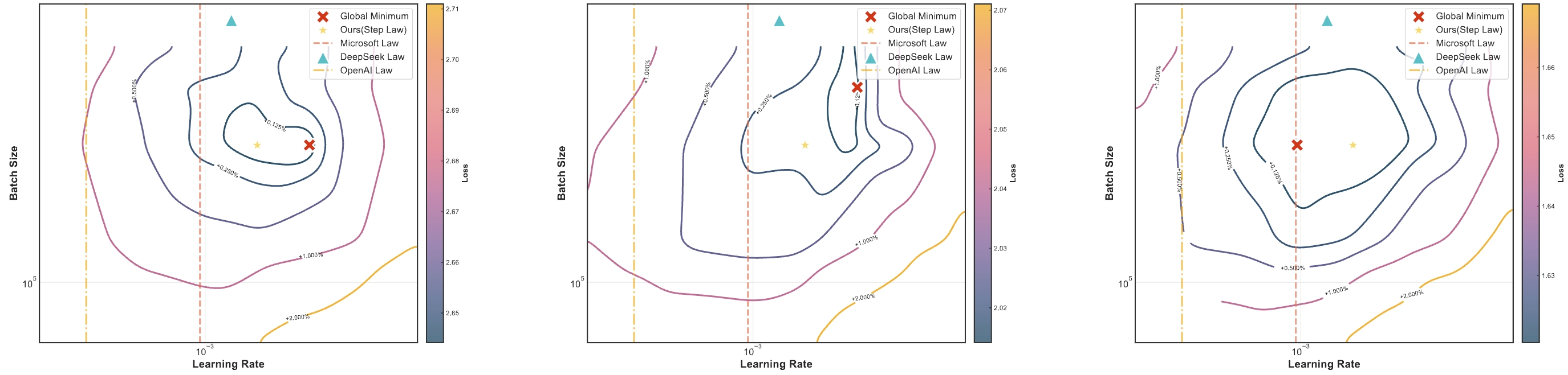
Our findings demonstrate remarkable accuracy, with estimated values on test sets deviating by only 0.09% from the globally optimal LLM performance identified through exhaustive search.

This research entails a significant computational investment, utilizing nearly one million NVIDIA H800 GPU hours to train 3,700 LLMs of varying sizes and hyperparameters from scratch, consuming approximately 100 trillion tokens in total. To support reproducibility and advance the field for LLM pre-training, we will progressively release all loss measurements and model checkpoints through our designated repository. The universal, plug-and-play optimal hyperparameter tool is provided for the community.

Step Law demonstrates that the optimal batch size $$B(D)$$ exhibits a primary dependence on dataset size $$D$$ , while the optimal learning rate $\eta(N, D)$ manifests a joint dependence on both model parameters $$N$$ and dataset size $$D$$ .

\begin{aligned} \eta(N, D) & = 1.79N^{-0.713}D^{0.307} \\ B(D) & = 0.58D^{0.571} \end{aligned}

Loss Landscape Convexity

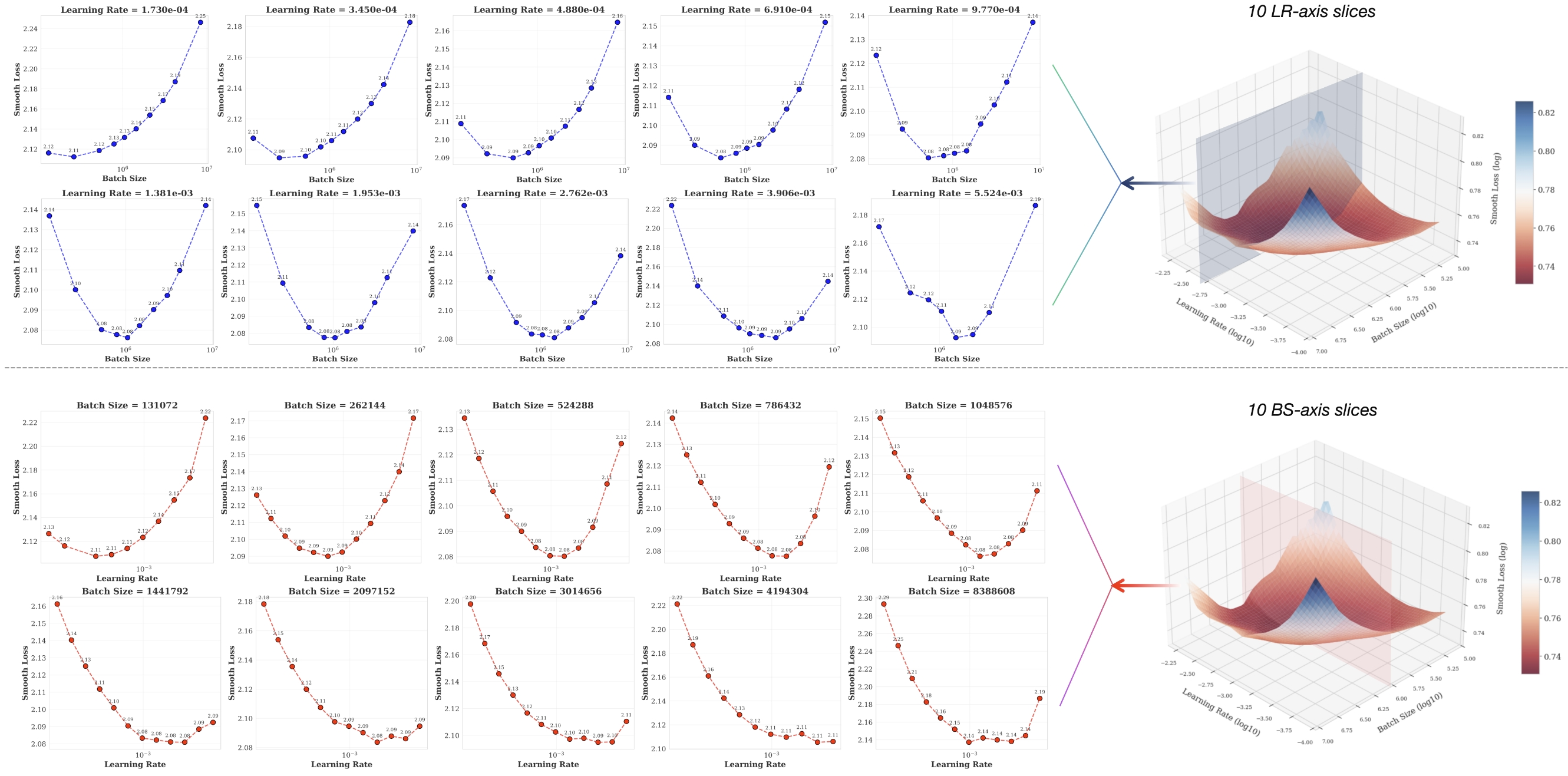
We discover and demonstrate the convexity property of the loss landscape under fixed parameter count and data size conditions. This provides fundamental insights into hyperparameter optimization.

**Figure 2. Learning Rate vs. Batch Size Loss Landscape Analysis for 1B Model (Trained on 100B Tokens) combining empirical scatter data (left) and reconstructed 3D surfaces (right):** Each solid point represents the converged Train Smoothed Loss from 120 small models trained from scratch. To visualize the convexity, researchers constructed a 3D coordinate system (right) with the x-axis as Learning Rate, y-axis as Batch Size, and z-axis as Loss. Horizontal and vertical cross-sections of this 3D space reveal loss patterns: the upper-left subplot shows the final converged Train Smoothed Loss under fixed Learning Rates with varying Batch Sizes, while the lower-left subplot displays the loss under fixed Batch Sizes with varying Learning Rates. A pronounced convexity is observed with a relatively flat region at the bottom of the convex basin suggesting that the optimal combinations of Learning Rate and Batch Size likely occupy a broad range rather than a single sharp minimum.

Generalization of the Step Law

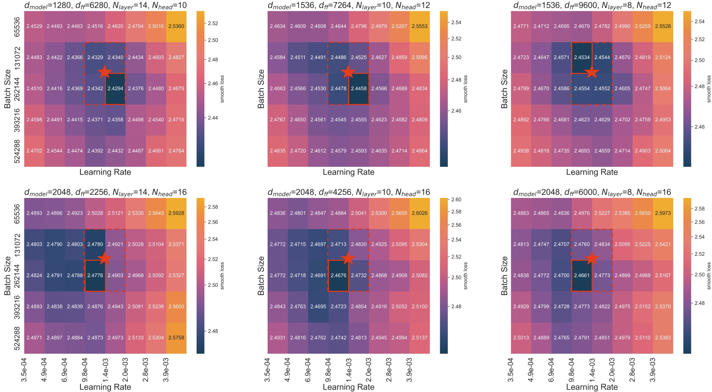
We conduct a comprehensive investigation into how different model architectures (specifically varying combinations of width and depth dimensions) influence scaling laws. Our findings demonstrate that Step Law exhibits a high degree of stability across all architectural configurations.

**Figure 3. Topological Invariance Across Varied Model Shape.** This figure demonstrates the topological invariance of optimal hyperparameters across different model shapes under fixed non-vocabulary parameter counts and training token budgets. Researchers systematically varied model architectures by adjusting layer counts (14/10/8 layers from left to right), hidden dimensions (1280/1536/2048), and six FFN multiples (FFN_media_dim/model_dim ranging from 1.1x to 6.25x). Red five-pointed stars denote predictions from the Step Law method, which consistently identifies near-global-minimum regions across all six model shapes. While the Step Law predictions remain stable, the positional shifts of the convex basin's bottom region across different architectures reveal shape-dependent variations in optimal hyperparameter configurations, despite preserved topological characteristics in the loss landscape.

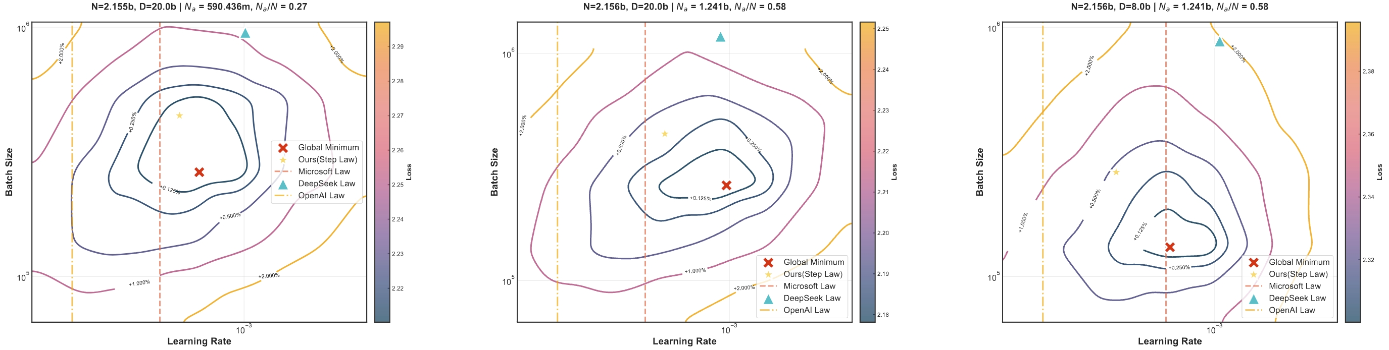
Besides, our research findings reveal that this scaling law not only applies to dense models but also generalizes effectively to MoE models with varying sparsity levels, demonstrating robust generalization capabilities.

**Figure 4. Validation loss landscapes of MoE models under varying sparsity ratios N_a/N.** The left panel shows low sparsity (NA/N = 0.27), the center illustrates moderate sparsity ( N_a/N = 0.58, D/N = 10), and the right depicts moderate sparsity with reduced training tokens (N N_a/N = 0.58, D/N = 4). Researchers trained 45 small models from scratch for each configuration across different sparsity levels and D/N ratios, totaling 495 distinct MoE models with varying sparsity, hyperparameters, and D/N settings, to derive ground-truth Global Minimum Train Smepothed Loss values. Except for one D/N = 1 experiment, Step Law predictions consistently fall within +0.5% of the global minimum across all configurations, with most within +0.25%, robustly validating the method. Detailed results are provided in the appendix.

Our experiment further validates the consistency of Step Law across diverse data distributions: whether in English-dominated, Chinese-English mixed, Code-English mixed, or Code-dominant, the Step Law demonstrates stable performance. This provides robust support for its practical applications in multilingual and multitask settings.

**Figure 5. Configuration Space Analysis under Different Data Recipes:** left panel shows bilingual data, center panel combines code and mathematical data, and right panel focuses on code-dominated data. Each configuration trained 45 models from scratch with identical settings except batch size and learning rate, totaling 135 models across three data distributions. The Global Minimum represents the ground-truth lowest Final Train Smoothed Loss obtained through grid search, while Step Law-predicted optimal batch sizes and learning rates consistently fall within +0.125% to 0.25% of the minimum loss across all data recipes.

Experimental Details

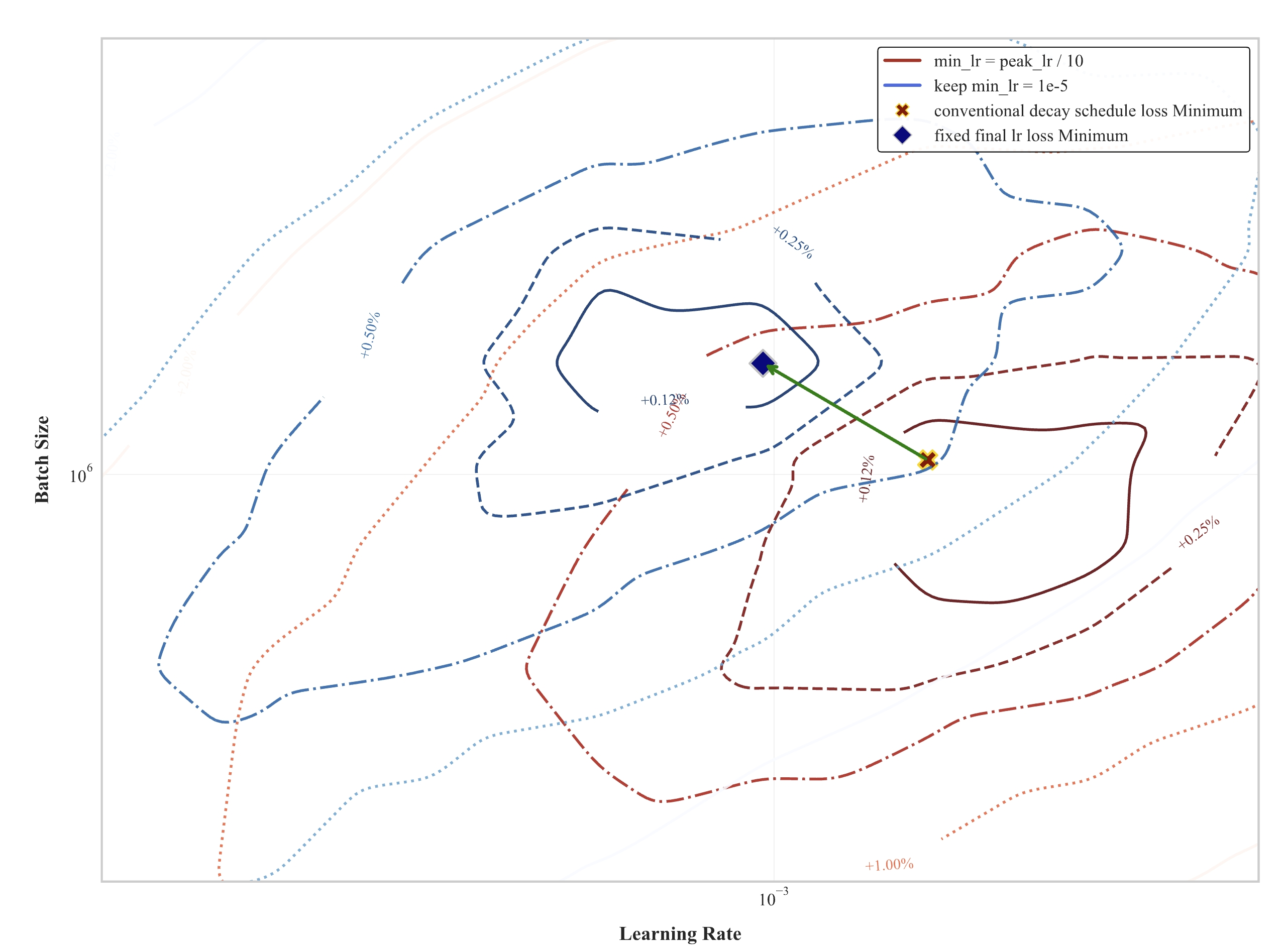
Our comparative analysis reveals that learning rate scheduling strategies significantly impact optimal hyperparameter selection. The experiment further uncovers critical distinctions between traditional learning rate decay and fixed minimum learning rate schemes.

**Figure 6. Comparison of learning rate schedules.** These contour plots illustrate two distinct learning rate schedules. **Blue contours** represent the *conventional decay schedule*, where the minimum learning rate min_lr is set to one-tenth of the maximum learning rate max_lr/10. **Red contours** depict our proposed *final learning rate schedule*, with a constant minimum learning rate of min_lr = 10^-5. All the contours present results from grid searches conducted over identical batch size/learning rate ranges using 120 independently trained models each. The red and blue Global Minimum markers denote ground-truth minimal Final Train Smoothed Loss values in their respective configurations. When switching to max_lr/10 settings, the blue markers shift **leftward (toward smaller learning rates) and upward (toward larger batch sizes)** in the parameter space. Absolute value comparisons reveal models with min_lr=1e-5 consistently achieve lower converged losses than those using max_lr/10 configurations. All ground-truth values corresponding to these experiments will be progressively open-sourced.

Through logarithmic transformation of power-law relationships into linear forms, parameters are fitted via the least squares method, with robustness enhanced through bootstrap sampling. We provide a precise predictive formula, establishing a theoretical foundation for hyperparameter configuration in LLMs pretraining.

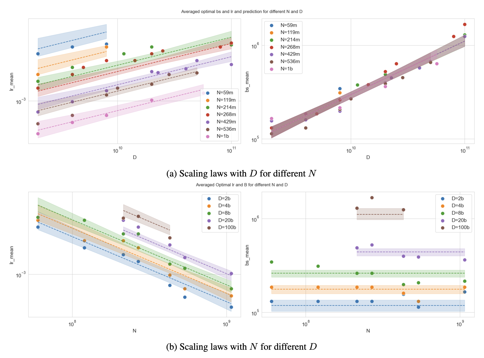
**Figure 7. (a) Scatter points indicate empirical optimal learning rate vs. batch size for model scale N; (b) Analogous results for dataset scale D.**
Curves show our hp-scaling law predictions, with shaded regions representing parameter uncertainty bounds from the sampling-based fitting strategy. Each data point in the figures represents between 45 and 120 independently trained models with distinct hyperparameters. Every plotted position corresponds to the optimal hyperparameter configuration (Optimal Learning Rate and Optimal Batch Size) identified through grid search under varying model sizes and data scales. Both plots use double logarithmic scaling (1912 training samples).

Step Law Tools

Open Source Roadmap

Live Progress Tracking

Milestone

Release Status

Predictable Scale Part I: Optimal Hyperparameter Scaling Law

ArXiv

Optimal Hyperparameter Tool

Tool

Training Dynamic of 3700 Models

Wandb

Train Smoothed Loss of 3700 Models

Github

Training Dynamics of 3700 Models

2025.3.30

Predictable Scale Part II

2025.4.15

Predictable Scale Part III

2025.5.15

BibTeX

@misc{li2025predictablescalei,
  title    = {Predictable Scale: Part I -- Optimal Hyperparameter Scaling Law in Large Language Model Pretraining}, 
  author   = {Houyi Li and Wenzheng Zheng and Jingcheng Hu and Qiufeng Wang and Hanshan Zhang and Zili Wang and Shijie Xuyang and Yuantao Fan and Shuigeng Zhou and Xiangyu Zhang and Daxin Jiang},
  year     = {2025},
  eprint   = {2503.04715},
  archivePrefix = {arXiv},
  primaryClass  = {cs.LG},
  url      = {https://arxiv.org/abs/2503.04715}, 
}